Tutorial
This chapter contains the installation instructions of BayHunter, followed by an example of how to set up and run an inversion. A minimalistic working example is shown in the Appendix. Furthermore, results from an inversion using synthetic data are shown and discussed. Be here also referred to the full tutorial including data files.
Requirements and installation
BayHunter is currently for a Python 2 environment (as of October, 2019). After installation of the required Python-modules, simply type the following to install BayHunter:
sudo python setup.py install
|
numerical computations |
|
plotting library |
|
merging PDFs |
|
configuration file |
|
BayWatch, inversion live-streaming |
|
C-extensions for Python |
The forward modeling codes for surface wave dispersion and receiver functions are already included in the BayHunter package and will be compiled when installing BayHunter. BayHunter uses a Python wrapper interfacing the
SURF96 routine from Herrmann and Ammon, 2002, and rfmini developed for BayHunter by
Joachim Saul, GFZ.
Setting up and running an inversion
Setting up the targets
As mentioned in Initialize the targets, BayHunter provides six target classes (four SWD and two RF),
which use two types of forward modeling plugins (SURF96,
rfmini). For both targets, the user may update the default forward
modeling parameters with set_modelparams (see Appendix). Parameters and default values are given in Table 1.
SWD |
mode = 1 |
1=fundamental mode, 2=1st higher mode, etc. |
RF |
gauss = 1.0 |
Gauss factor, low pass filter |
water = 0.001 |
water level stabilization |
|
p = 6.4 |
slowness in deg/s |
|
nsv = |
near surface velocity in km/s for computation
of incident angle (trace rotation). If
|
If the user wants to implement own forward modeling code, a new forward modeling class for it is needed. After normally initializing a target with BayHunter, an instance of the new forward modeling class must be initialized and passed to the update_plugin method of the target. If an additional data set is wished to be included in the inversion, i.e., from a non pre-defined target class, a new target class needs to be implemented, additionally to the forward modeling class that handles the synthetic data computation. For both, the forward modeling class and the new target class, a template is stored on the GitHub repository. It is important that the classes implement specifically named methods and parameters to ensure the correct interface with BayHunter.
Setting up parameters
Each chain will be initialized with the targets and with parameter dictionaries. The model priors and inversion parameters that need to be defined are listed with default values in Table 2, and are explained below in detail.
vs |
= (1, 5) |
nchains |
= 3 |
z |
= (0, 60) |
\(i ter_ {burnin}\) |
= 4096 |
layers |
= (1, 20) |
\(i te r_{main}\) |
= 2048 |
vpvs |
= (1.5, 2.1) |
acceptance |
= (40, 45) |
mantle \(^1\) mohoest \(^2\) |
= = |
propdist \(^3\) |
= (0.015, 0.015, 0.005, 0.015, 0.005) |
\(r_ {RF}\) |
= (0.35, 0.75) |
thickmin |
= 0. |
\(\sigma _{RF}\) |
= (1e-5, 0.05) |
lvz |
= |
\(r_ {SWD}\) |
= 0. |
hvz |
= |
\(\sigma _{SWD}\) |
= (1e-5, 0.1) |
rcond |
= |
\(^1\) i.e., (vs\(_m\), vpvs\(_m\)), e.g., (4.2, 1.8) |
station |
= ’test’ |
|
\(^2\) i.e., (z\(_{mean}\), z\(_{std}\)), e.g., (40, 4) |
savepath |
= ’results/’ |
|
\(^3\) i.e., (vs, z\(_{move}\), vs\(_{birth/death}\), noise, vpvs) |
maxmodels |
= 50 000 |
|
The priors for the velocity-depth structure include \(\mathrm{V_S}\) and depth, the number of layers, and average crustal \(\mathrm{V_P}\)/\(\mathrm{V_S}\). The ranges as given in Table 2 indicate the bounds of uniform distributions. \(\mathrm{V_P}\)/\(\mathrm{V_S}\) can also be given as a float digit (e.g., 1.73), indicating a constant value during the inversion. The parameter \(layers\) does not include the underlying half space, which is always added to the model. A mantle condition (vs\(_m\), vpvs\(_m\)), i.e., a vs\(_m\) threshold beyond which \(\mathrm{V_P}\) is computed from vpvs\(_m\), can be chosen if appropriate. There is also the option to give a single interface depth estimate through \(mohoest\). It can be any interface, but the initial idea behind was to give a Moho estimate. As explained in Initialize a model, this should only be considered for testing purposes. Each noise scaling parameter (\(r\), \(\sigma\)) can be given by a range or a digit, corresponding to the bounds of a uniform distribution (the parameter is inverted for) or a constant value (unaltered during the inversion), repectively.
For surface waves, the exponential correlation law (Eq. (3)) is a realistic estimate of the correlation between data points and is automatically applied. For receiver functions, the assumed correlation law should be Gaussian (Eq. (4)), if the RFs are computed using a Gaussian filter, and exponential, if the RFs are computed applying an exponential filter. The inversion for \(r_{RF}\) is viable for the latter, however, not for the Gaussian correlation law as of computational reasons (see Computation of model likelihood). Only if \(r_{RF}\) is estimated by giving a single digit, the Gaussian correlation law is considered. Otherwise, if given a range for \(r_{RF}\), the exponential correlation law is used. Note that the estimation of \(r_{RF}\) using the exponential law during an inversion, may not lead to correct results if the input RF was Gaussian filtered.
Nevertheless, \(r_{RF}\) can be estimated, as it is dependent on the sampling rate and the applied Gaussian filter width. Figure 5 shows an application of the BayHunter implemented tool to estimate \(r_{RF}\). You will find a minimalistic code example in the Appendix and an executable file with plenty of comments in the tutorial folder of the repository.
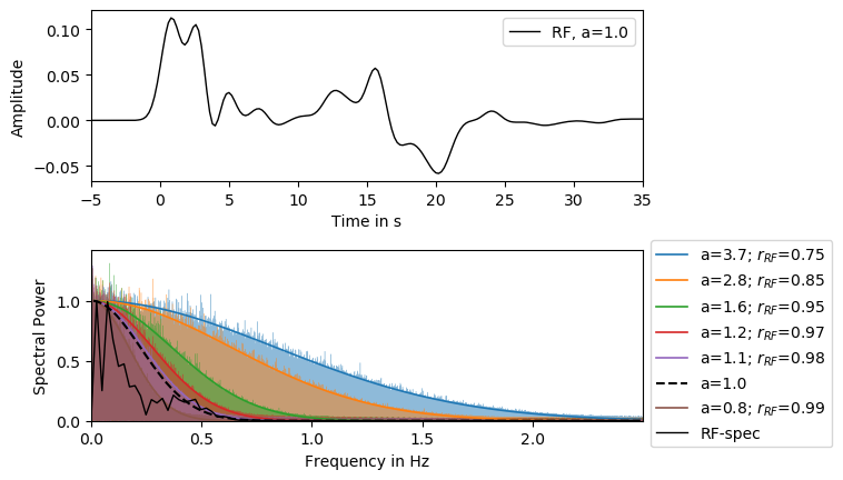
Fig. 5 Visual estimation of \(r_{RF}\). Top: Synthetic receiver function from a 3-layer crustal model, applying a Gaussian low pass filter with the Gaussian factor \(a\) =1. Bottom: Frequency spectrum of synthetic receiver function (solid black) and Gaussian filter with \(a\) =1 (dashed black). Transparently colored areas correspond to the spectra of large sample draws of synthetic Gaussian correlated noise using different values of \(r_{RF}\). The solid colored lines represent the Gaussian curves matching the data ‘envelope’. The legend displays corresponding \(r_{RF}\) and \(a\) values. For the given receiver function, a proper estimate of \(r_{RF}\) is 0.98.
If \(r_{RF}\) is too large (i.e., very close to 1), \(R^{-1}\) becomes instable and small eigenvalues need to be suppressed. The user can define the cutoff for small singular values by defining \(rcond\). Singular values smaller than \(rcond\) x the largest singular value (both in modulus) are set to zero. \(rcond\) is not ascribed to the prior dictionary, but to the inversion parameter dictionary (see configuration file).
The inversion parameters can be subdivided into three categories: (1) actual inversion parameters, (2) model constraints and (3) saving options. Parameters to constrain the inversion are the number of chains, the number of iterations for the burn-in and the main phase, the initial proposal distribution widths, and the acceptance rate. A large number of chains is preferable and assures good coverage of the solution space sampling, as each chain starts with a randomly drawn model only bound by the priors. The number of iterations should also be set high, as it can benefit, but not guarantee, the convergence of the chain towards the global likelihood maximum. The total amount of iterations is \(iter_{total} = iter_{burnin} + iter_{main}\). We recommend to increase the ratio towards the iterations in the burn-in phase (i.e., \(iter_{burnin}>iter_{main}\)), so a chain is more likely to have converged when entering the exploration phase for the posterior distribution.
The initial proposal distributions, i.e., Gaussian distributions centered at zero, for model modifications, must be given as standard deviations according to each of the model modification methods (Propose a model). The values must be given as a vector of size five, the order representing following modifications: (1) \(\mathrm{V_S}\), (2) depth, (3) birth/death, (4) noise, and (5) \(\mathrm{V_P}\)/\(\mathrm{V_S}\). The first three distributions represent \(\mathrm{V_S}\)-depth model modifications referring to alterations of \(\mathrm{V_S}\)(1,3) and z (2) of a Voronoi nucleus. There is one proposal distribution for both noise parameters \(r\) and \(\sigma\) (4) and one for \(\mathrm{V_P}\)/\(\mathrm{V_S}\)(5).
If the proposal distributions were constant, the percentage of accepted proposal models would decrease with ongoing inversion progress, i.e., the acceptance rate decreases at the expense of an efficient sampling. To efficiently sample the parameter space, an acceptance rate of \(\sim\)40–45 % is forced for each proposal method by dynamically adapting the width of each proposal distribution. We implemented a minimum standard deviation of 0.001 for each proposal distribution.
The most accepted model modifications are (1) and (2); their acceptance rates get easily forced to the desired percentage without even coming close to the defined minimum width of a proposal distribution. Birth and death steps, however, barely get accepted after an initial phase of high acceptance; if not limiting the proposal distribution width to a minimum, the standard deviations for (3) will get as small as \(10^{-10}\) km/s and smaller to try to keep the acceptance rate up. However, as discussed in Propose a model, the distribution width does not in the first place influence the model-modification, but the added or removed Voronoi nucleus. Models modified by birth and death steps will naturally not be accepted very often and even less the further the inversion progresses. Therefore, the overall acceptance rate is stuck with a specific level below the forced rate. An estimate of the actual overall acceptance rate can be made, assuming a realistic acceptance for the birth and death steps, e.g., 1 %. A user given target rate of 40 % for each method would give an actual overall acceptance rate of \(\sim\)3 %. (\(\rightarrow\) 6 methods, 4 reach 40 %, 2 only 1 % = 30 % over all.) The target acceptance rate must be given as an interval.
There are three additional conditions, which might be worthwhile to use
to constrain the velocity-depth model. However, using any of them could
bias the posterior distribution. The user is allowed to set a minimum
thickness of layers. Furthermore low and high velocity zones can be
suppressed. If not None, the value for \(lvz\) (or \(hvz\))
indicates the percentage of allowed \(\mathrm{V_S}\) decrease (or
increase) from each layer of a model relative to the underlying layer.
For instance, if \(lvz\)=0.1, then a drop of \(\mathrm{V_S}\)
by 10 %, but not more, to the underlying layer is allowed. As
\(\mathrm{V_S}\) naturally increases with depth, and the algorithm
only compares each layer with the layer underneath, the \(hvz\)
criteria should only be used if observing extreme high velocity zones in
the output. Otherwise sharp (but real) discontinuities could be smoothed
out, if chosen too small. The \(lvz\) and \(hvz\) criteria will
be checked every time a velocity-depth model is proposed and the model
will be rejected if the constraints are not fulfilled.
The saving parameters include the \(station\), \(savepath\) and \(maxmodels\). The \(station\) name is optional and is only used as a reference for the user, for the automatically saved configuration file after initiation of an inversion. \(savepath\) represents the path where all the result files will be stored. A subfolder data will contain the configuration file and all the SingleChain output files, the combined posterior distribution files and an outlier information file. \(savepath\) also serves as figure directory. \(maxmodels\) is the number of p2-models that will be stored from each chain.
Running an inversion
The inversion will start through the optimizer.mp_inversion command with the option to chose the number of threads, \(nthreads\), for parallel computing. By default, \(nthreads\) is equal to the number of CPUs of the user’s PC. One thread is occupied if using BayWatch. Ideally, one chain is working on one thread. If fully exhausting the capacity of a 8 CPUs PC, give \(nthreads\)=8 and \(nchains\)=multiple of \(nthreads\) or (\(nthreads\)-1) if using BayWatch. This would cause \(nthreads\)(-1) chains to run parallel at all times, until \(nchains\) are worked off.
The speed of the inversion will not increase by choosing a larger \(nthreads\). In fact, the speed is determined by the number of CPUs. If, for instance, the user doubles \(nthreads\), the number of chains running parallel at once is also double, but the chains queue for some non-threadable computations blocking one CPU at a time, so each chain runs half the speed. To decrease \(nthreads\) offers a possibility to minimize the workload for a PC and that it is still accessible for other tasks during an inversion.
Although having access to a cluster, inversions were also performed on a single work station to determine the duration of an inversion with standard PC equipment (e.g., Memory: 16 GB, Processor model: 3.60 GHz x 8 cores). The runtime is not only dependent on the PC model, but also on the number of chains and iterations, and the number of layers of the actual velocity-depth structures, which directly influences the computational time of the forward modeling. The inversion for the example given in Testing with synthetic data with 21 chains, 150,000 iterations and models with 3–10 layers, took 20.4 minutes; so each batch of 7 chains took 7 minutes.
Another argument to set when starting an inversion is \(baywatch\). If set to True, model data will be send out with an interval of \(dtsend\)=0.5 s and can be received by BayWatch until the inversion has finished.
Testing with synthetic data
A set of test data was computed with the BayHunter.SynthObs module, which provides methods for computing receiver functions (P, S), surface wave dispersion curves (Love, Rayleigh, phase, group), and synthetic noise following the exponential or the Gaussian correlation law. We computed the P-RF and the fundamental mode SWD of the Rayleigh wave phase velocity from a six-layer model including a low velocity zone. We computed non-correlated noise for SWD and Gaussian correlated noise for the RF with values for \(r\) and \(\sigma\) as given in Table 3 (true). Noise and synthetic data were then added to create observed data. An example script, including these steps, can be found in the Appendix and the online repository.
vs |
= (2, 5) |
nchains |
= 21 |
z |
= (0, 60) |
\(i ter_{burnin}\) |
= 100,000 |
layers |
= (1, 20) |
\(i ter_{main}\) |
= 50,000 |
vpvs |
= (1.5, 2.1) |
acceptance |
= (50, 55) |
\(r_{RF}\) |
= 0.92 |
propdist |
= (0.005, 0.005, 0.005, 0.005, 0.005) |
\(\sigma_ {RF}\) |
= (1e-5, 0.05) |
rcond |
= 1e-6 |
\(r_{SWD}\) |
= 0. |
station |
= ’st6’ |
\(\sigma_ {SWD}\) |
= (1e-5, 0.1) |
Two targets (PReceiverFunction, RayleighDispersionPhase) were initialized with the “observed” data and combined to a BayHunter.JointTarget object. The latter and the two parameter dictionaries of model priors and inversion parameters (Table 3) were passed to the Optimizer. Parameters that were not defined fall back to the default values. We purposely show a run with only 150,000 iterations to visualize the convergence of different chains and the outlier detection method. The inversion finished after 20 minutes, saving and plotting methods were applied afterwards.
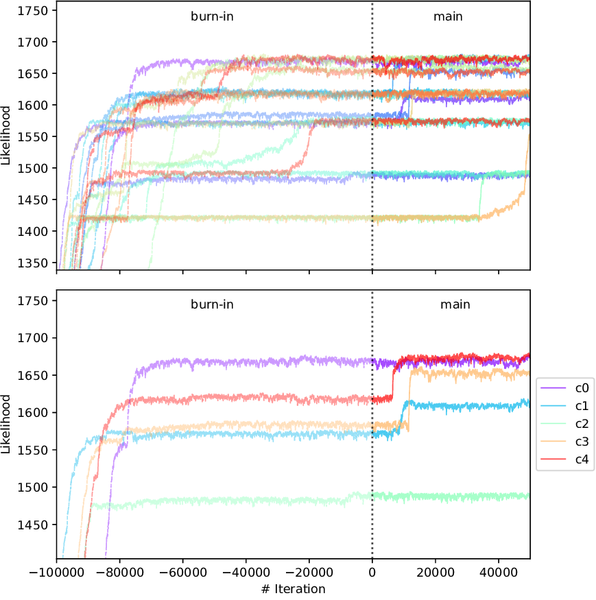
Fig. 6 Development of likelihood over iteration for all 21 chains (top) and a small selection of chains (bottom).
Figure 6 shows the likelihood development over the iterations for all and for a selection of chains. A strong increase of likelihood can be observed at the first iterations in the burn-in phase, converging towards a stable value with increasing number of iteration. Some chains reached the final likelihood plateau in the burn-in phase (e.g., \(c0\)), some within the posterior sampling phase (e.g., \(c4\)), and some did not converge at all (\(c2\)). The chain \(c2\) (also \(c1\) and \(c3\)) had a good chance of reaching the maximum likelihood, if the small number of iterations would not have stopped the exploration at this early stage. However, the number of iterations cannot be eternal; in any case it is necessary to compare the convergence level of the chains.
Here, we defined a 0.02 deviation condition for outliers. With a maximum median posterior likelihood of 1674 (\(c13\)), the likelihood threshold is 1640, which declared 13 chains with deviations of 0.032–0.159 as outliers (see Table 4). In a real case inversion, the number of iterations should be much higher, and the number of outlier chains is small. The detected outlier chains will be excluded from the posterior distribution.
c1 |
0.039 |
c6 |
0.061 |
c9 |
0.059 |
c15 |
0.150 |
c19 |
0.059 |
c2 |
0.111 |
c7 |
0.033 |
c10 |
0.150 |
c16 |
0.033 |
||
c5 |
0.032 |
c8 |
0.109 |
c14 |
0.033 |
c17 |
0.033 |
Figure 7 shows the current \(\mathrm{V_S}\)-depth models from different chains and corresponding data fits (same chains as in Figure 6, bottom). Chains \(c1\) and \(c2\) show the worst data fits; they were declared as outliers. The other chains (\(c0\), \(c3\), \(c4\)) show a reasonably good data fit with very similar velocity models. Chains \(c0\) and \(c4\) already found a six-layer model, \(c3\) found a five-layer model averaging the low velocity zone.
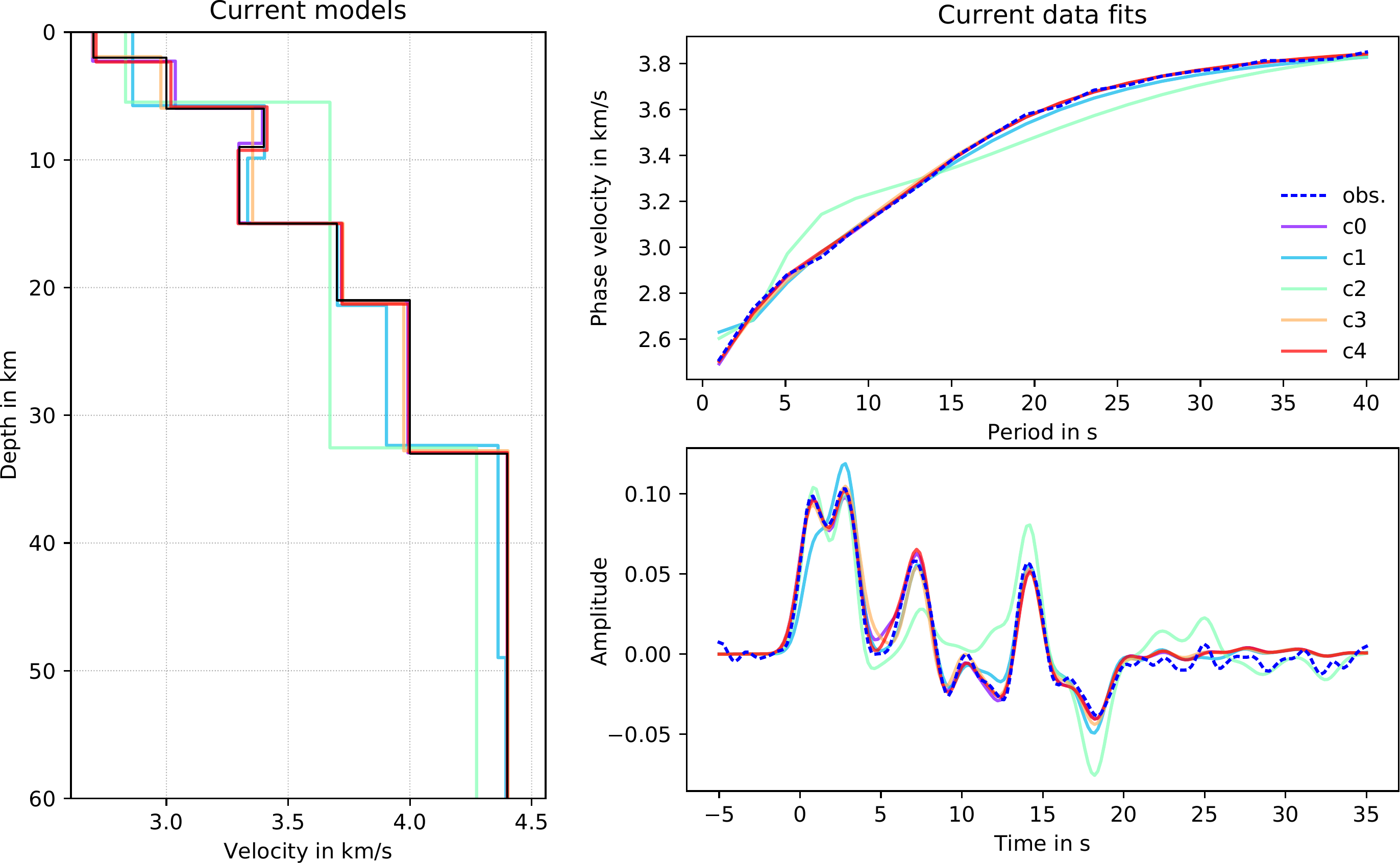
Fig. 7 Current velocity-depth models and data fits of corresponding SWD and RF data from different chains with likelihoods as illustrated in Figure 6 (bottom). The black line (left) is the synthetic \(\mathrm{V_S}\)-depth structure.
The posterior distribution of the eight converged chains, containing 100,000 models, are illustrated in Figure 8. The mean (and mode) posterior \(\mathrm{V_S}\)-depth structure images the true model very well, including the low velocity zone. The number of layers is determined to be most likely six. The \(\sigma\) distributions of both, RF and SWD show a Gaussian shape, inhering a tail of higher values from models of chains that only converged within the exploration phase of the inversion (e.g., \(c3\) and \(c4\)). The distribution of \(\sigma_{SWD}\) already represents a good estimate, slightly overestimated, which falls back to the number of iterations. Tests with more iterations show that the median of \(\sigma_{SWD}\) is in perfect agreement with the true value.
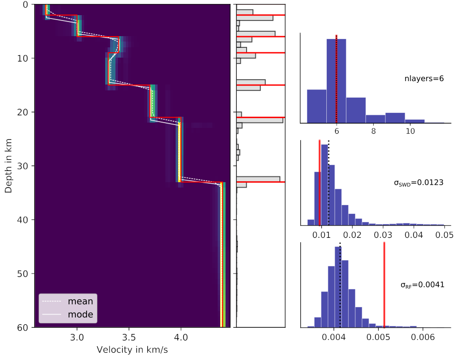
Fig. 8 Recovered posterior distributions of \(\mathrm{V_S}\), interface depth, number of layers, and noise level for synthetic data. Red lines indicate the true model, as given in Table 3. The posterior distribution is assembled by 100,000 models collected by 8 chains.
\(\sigma_{RF}\) is underestimated, which theoretically means that noise was interpreted as signal and receiver function data is overfitted. The difference to SWD is the type of noise correlation (= Gaussian) and the assumption of the correlation \(r\) of data noise (\(r\neq0\)). We computed synthetic RF data applying a Gaussian lowpass filter with a Gaussian factor of 1. Separately, noise was generated randomly with a correlation \(r\) estimated to represent the applied Gauss filter, and added to the synthetic data. The random process of generating noise does not output a noise vector which exactly matches the given values of \(r\) and \(\sigma\). If only drawing one single realization with a determined amount of samples from the multivariate normal distribution may produce deviations from the targeted \(r\) and \(\sigma\). From the generated noise the true \(\sigma\) can be computed by the standard deviation. However, the true \(r\) is not easy to reconstruct. Assuming a wrong \(r\) for the covariance matrix of noise cannot lead to the correct \(\sigma\).
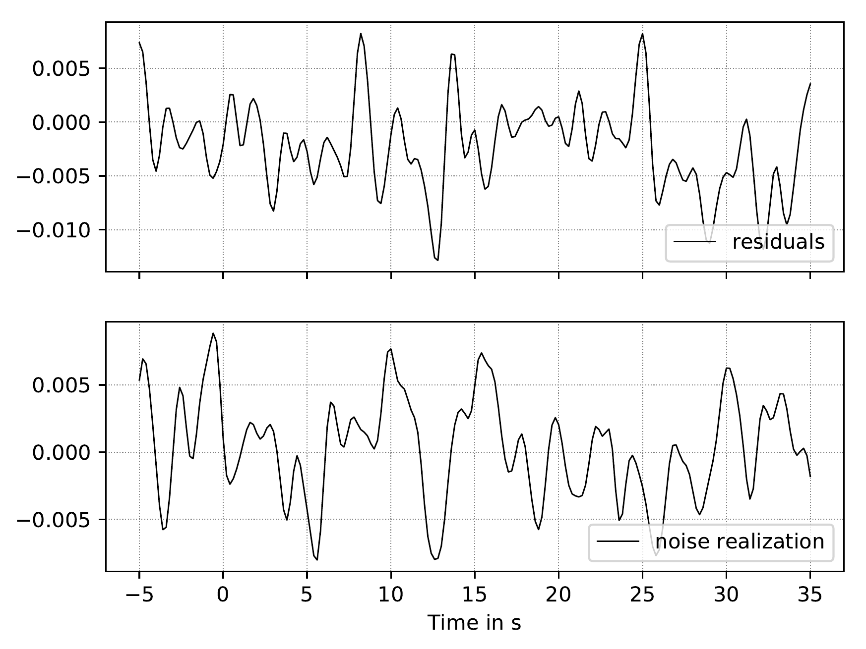
Fig. 9 Comparison of residuals of the best fitting RF model and one realization of noise through \(C_e^{RF}\) for receiver functions. Both noise vectors are of coherent appearance in frequency and amplitude, hence, the estimate of \(r_{RF}\) is appropriate.
It is possible to clarify whether the assumed correlation parameter \(r\) is in tendency correct. Figure 9 shows a comparison of (1) the RF data residuals of the best fitting model and (2) one realization of noise with the given correlation \(r\) and the estimated \(\sigma_{RF}\); both noise vectors should be of coherent appearance in frequency and amplitude, if the estimate of \(r_{RF}\) is appropriate.