Introduction

Bayesian inversion is becoming more and more popular for several years and it has many advantages compared to conventional optimization approaches. While other methods often are more constrained and favor one best model based on the least misfit, an inversion after Bayes theorem is based on the model’s likelihood and results in probability distributions for each parameter of the model. The inversion result is represented by a collection of models (posterior distribution) that are consistent with the data and with the selected model priors. They image the solution space and disclose uncertainties and trade-offs of the model parameters.

No open-source tools were available that suited our purpose of a joint inversion of SWD and RF after Bayes using a Markov chain Monte Carlo (McMC) sampling algorithm, and solve for the velocity-depth structure, the number of layers, the noise parameters, and the average crustal \(\mathrm{V_P}\)/\(\mathrm{V_S}\) ratio. So it was natural to take care of this. We developed BayHunter to serve that purpose, and BayWatch, a module that allows to live-stream the inversion while it is running.

Bayes theorem

Bayes theorem (Bayes, 1763) is based on the relationship between inverse conditional probabilities. Assuming observed data \(d_{obs}\) and a model \(m\); the probability that we observe \(d_{obs}\) given \(m\) is \(p(d_{obs}|m)\), and the probability for \(m\) given \(d_{obs}\) is \(p(m|d_{obs})\). Both occurrences are also dependent on the probability that \(m\) or \(d_{obs}\) is given, i.e., \(p(m)\) and \(p(d_{obs})\).

The inverse conditional probability that both events occur, is given by:

\[p(m|d_{obs}) p(d_{obs}) = p(d_{obs}|m) p(m)\]

As \(d_{obs}\) is known as the evidence, i.e., the measurements, Bayes theorem can be rewritten to:

(1)\[% posterior $\propto$ likelihood x prior p(m|d_{obs}) \propto p(d_{obs}|m) p(m)\]

\(p(m|d_{obs})\) is the posterior distribution, \(p(d_{obs}|m)\) is called the likelihood, and \(p(m)\) is the prior probability distribution.

Markov chain Monte Carlo

Markov chain Monte Carlo describes a sampling algorithm for sampling from a probability distribution. This algorithm is a combination of Monte Carlo, a random sampling method, and Markov chains, assuming a dependency between the current and the previous sample. For the exact implementation of the algorithm, see section Algorithm.

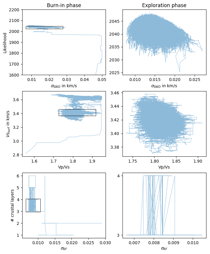
Fig. 1 McMC sampling scheme for one chain progressing through the parameter space. Left and right columns show iterations of the burn-in (first phase) and exploration phase (second phase), respectively, with the black box framing the exploration region as shown in the right column. Illustrated parameters are the likelihood and noise amplitude \(\sigma_{SWD}\), surface vs and vp/vs, and number of crustal layers and noise amplitude \(\sigma_{RF}\). The top panels reflect the optimization process based on the likelihood, while the lower panels show the parameter trade-off. Example taken from station SL10 in Sri Lanka.

Figure 1 shows a real data example from a station in Sri Lanka (SL10), following the evolution of one chain through the model parameter space. Parameters are shown in couples, but note that the parameter space is multidimensional. In the burn-in phase (left column) the chain starts at a random parameter combination in the solution space and progresses with ongoing iterations towards an optimum, based on the likelihood. In the second phase (right column) the chain has already reached its exploration region and samples the posterior distribution.

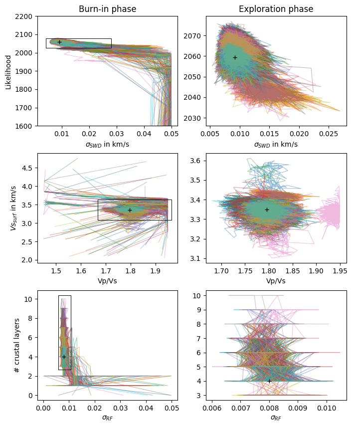
Fig. 2 McMC sampling scheme for one hundred chains progressing independently through the parameter space. Same parameters and parameter space as illustrated in Figure 1. Black cross shows the median from the complete posterior distribution (exploration phase). Example taken from station SL10 in Sri Lanka.

Figure 2 shows one hundred independent chains exploring the same parameter space. Each chain starts with a different random model, yet most chains converge to the same exploration region for sampling the posterior distribution. There are still chains (e.g., the two rose colored ones in the middle panel) that have not converged into the optimum zone when entering the exploration phase. If those chains do not converge to that optimum zone within the second phase, they probably represent outlier chains (or secondary minima) and should not be considered for the posterior distribution.