Algorithm
BayHunter is a tool to perform McMC transdimensional Bayesian inversion of SWD and RF, solving for the velocity-depth structure, the number of layers, noise scaling parameters (correlation, sigma), and average crustal \(\mathrm{V_P}\)/\(\mathrm{V_S}\). The inversion algorithm uses multiple independent Markov chains and a random Monte Carlo sampling to find models with the highest likelihood.
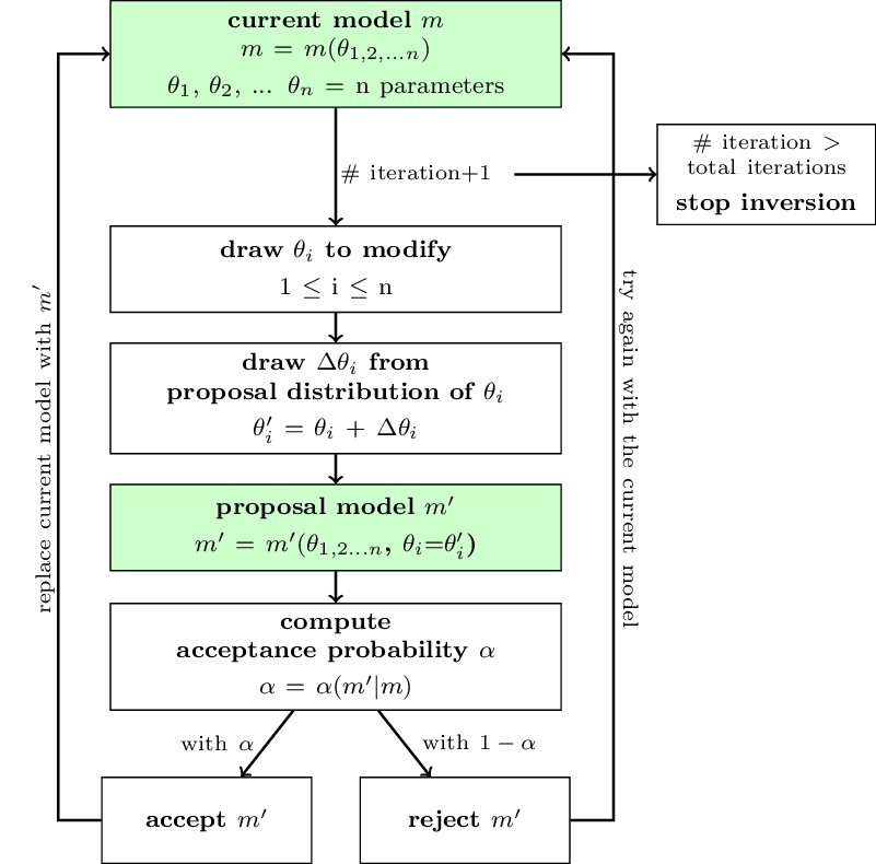
Fig. 3 Schematic workflow of an McMC chain sampling the parameter space. The posterior distribution includes all accepted models of a chain after a chosen number of iterations.
How each chain is progressing through the parameter space is schematically illustrated in Figure 3. Each chain contains a current model. In each iteration a new model will be proposed, considering a proposal distribution, by modification of the current model. The acceptance probability is computed based on the prior, proposal and posterior ratios from proposal to current model. A proposed model gets accepted with a probability equal to the acceptance probability, i.e., if the likelihood of the proposed model is larger than the one of the current model, it gets accepted; but also models that are less likely than the current model get accepted with a small probability, which prevents the chain to get stuck in a local maximum. If a proposal model gets accepted, it will replace the current model; if not, the proposal model gets rejected and the current model stays unmodified. This process will be repeated for a defined number of iterations. Each accepted model of the exploration phase contributes to the posterior distribution of the parameters.
Equations given below are reduced to the number of those required in BayHunter, and will not be fully deduced. For mathematical derivations and details be referred to Bodin (2010) and Bodin et al. (2012), which inspired the idea of BayHunter and on which our algorithm is based on.
The Optimizer and Chain modules
The BayHunter.mcmcOptimizer manages the chains in an overarching module. It starts each single chain’s inversion and schedules the parallel computing. Each chain and its complete model data can be accessed (in the Python environment) after the inversion has finished. Before the optimizer initializes the chains, a configuration file will automatically be saved, which simplifies the process of illustrating results after an inversion.
Each BayHunter.SingleChain explores the parameter space independently and collects samples by following Bayes theorem (Eq. (1)). A chain has multiple tasks, which are described below in detail and begin with the random initialization of a starting model.
Initialize the targets
The first step towards an inversion is to define the target(s). Therefore, the user needs to pass the observed data to the designated BayHunter target type. For surface wave dispersion, period-velocity observables must be assigned to the class that handles the corresponding data (RayleighDispersionPhase, RayleighDispersionGroup, LoveDispersionPhase, LoveDispersionGroup). They default into the fundamental wave mode. Additionally, uncertainties can be attributed, which later control the weighting of each period. For receiver functions, observed time-amplitude data must be assigned to the PReceiverFunction (or SReceiverFunction) class from BayHunter.Targets. Parameters (Gauss filter width, slowness, water level, near surface velocity) for forward modeling should be updated, if the default values differ from the values used for RF computation.
Each of the target classes comes with a forward modeling plugin, which
is easily exchangeable. For surface waves, a quick Fortran routine based
on SURF96 (Herrmann and Ammon, 2002) is
pre-installed. For receiver functions, the pre-installed routine is based on rfmini
(Joachim Saul, GFZ). Also other targets can be defined.
Parametrization of the model
The model includes the velocity-depth structure and the noise parameters of the observed data.
Velocity-depth structure
The velocity-depth model is parametrized through a variable number of Voronoi nuclei, the position of each is given by a depth and a seismic shear wave velocity (\(\mathrm{V_S}\)). A model containing only one nucleus represents a half-space model, two nuclei define a model with one layer over a half-space and so on. The layer boundary (depth of an interface) lies equidistant between two nuclei. The advantage to use Voronoi nuclei over a simple thickness-velocity representation is, that one model can be parametrized in many different ways. However, a set of Voronoi nuclei defines only one model. The number of layers in a model is undefined and will be inverted for (transdimensional). \(\mathrm{V_P}\) is computed from \(\mathrm{V_S}\) through \(\mathrm{V_P}\)/\(\mathrm{V_S}\), which is chosen by the user to be constant, or an additional parameter to solve for.
Covariance matrix of data noise
The noise level is defined by two parameters, the correlation \(r\) (i.e., the correlation of adjacent data points) and the noise amplitude \(\sigma\). Both \(r\) and \(\sigma\) are treated as unknown and can be estimated during the inversion. They are the part of the observed data that can not be fitted. Hence, the observed data vector can be described as
where \(n\) is the size of the vector and \(\epsilon(i)\) represents errors that are distributed according to a multivariate normal distribution with zero mean and covariance \(C_e\).
The covariance matrix \(C_e\) is dependent on \(\sigma\) and \(R\), which is the symmetric diagonal-constant or Toeplitz matrix.
We consider two correlation laws for the correlation matrix \(R\). The exponential law is given by
and the Gaussian law by
where \(r = c_1\) is a constant number between 0 and 1. In BayHunter we consider the exponential correlation law for surface wave dispersion, and both the exponential and the Gaussian law for receiver functions.
Initialize a model
For each chain, the initial model parameters (starting model) are drawn from the uniform prior distributions. These are, for the velocity-depth structure, the distributions of \(\mathrm{V_S}\), depth, the number of layers and the average crustal \(\mathrm{V_P}\)/\(\mathrm{V_S}\). The initial model has a number of layers equal to the minimum value of the corresponding prior distribution. If set to 0, a half-space model will be drawn, if set to 1 a one layer over a half-space model represents the initial model and so on. The initial number of layers determines how many Voronoi nuclei will be drawn, i.e., how many pairs of \(\mathrm{V_S}\) and depth. If a velocity-depth model was drawn, \(\mathrm{V_P}\) will be computed from \(\mathrm{V_P}\)/\(\mathrm{V_S}\), which was either drawn hitherto or given as constant by the user. If appropriate, the user may wish to select a mantle specific \(\mathrm{V_P}\)/\(\mathrm{V_S}\), by also assuming a \(\mathrm{V_S}\) to distinguish the mantle from the crust. The density is computed by \(\rho = 0.77+0.32 V_P\) (Berteussen, 1977).
It is possible to give a single interface depth estimate (it can be any interface, e.g., the Moho). The estimate includes a mean and a standard deviation of the interface depth. When initializing a model - and only if an estimate was given - an interface depth is drawn from the given normal distribution and two nuclei will be placed equidistant to the interface. If the initial model only consists of a half-space, the interface estimate will be ignored. Giving an estimate can help the chains to converge more quickly, e.g., if computation capacity is limited, but might generate biased posterior distributions.
Each target has two noise scaling parameters (\(r\), \(\sigma\)). The user needs to define the prior distributions for the overarching target type, i.e., SWD and RF, nevertheless, each target will sample an own posterior distribution. Single noise parameters can also be set constant during an inversion by giving a single digit, instead of a range. Initial values are then the given digits, and/or will be drawn from the prior range.
The drawn starting model automatically is assigned as the current model of the chain. The corresponding likelihood is computed. This model is also the first model in the model chain that gets collected for the burn-in phase.
Computation of model likelihood
The likelihood is an estimate of the probability of observing the measured data given a particular model \(m\). It is an important measure for accepting and declining proposal models. The likelihood function is
where \(\Phi(m)\) is the Mahalanobis distance (Mahalanobis, 1936), i.e., the multidimensional distance between observed \(d_{obs}\) and estimated \(g(m)\) data vectors.
As the likelihood often results in very small numbers, the log-likelihood is preferred.
The computation of the likelihood needs the inverse \(C_{e}^{-1}\) and determinant \(|C_e|\) of the covariance matrix. For the exponential correlation law (Eq. (3)), the covariance matrix is described by
\(C_{e}^{-1}\) and \(|C_e|\) can be solved through linear algebra, and are given by the analytical forms
and
These can be easily constructed and quickly computed in the Python language. Obviously, if the correlation of noise \(r=0\), the matrices \(R\) (Eq. (2)) and \(R^{-1}\) are simply formed by the diagonal matrix, and the determinant is given by \(\sigma^{2n}\). This is the default case for surface wave dispersion. If the dispersion measurements were assigned uncertainty values, then \(\sigma^{2}\) is weighted by the relative uncertainties.
For receiver functions, unless they are computed utilizing an exponential filter, the Gaussian correlation law (Eq. (4)) should be considered. In this case \(C_{e}^{-1}\) and \(|C_e|\) cannot be solved analytically and the numerical computation of these is necessary. Considering a numerical computation each time a noise parameter is perturbed will increase the computation time tremendously. A trick to speed up the computation is accompanied by estimating \(r\) priorly and keeping it constant during the inversion. The equations
and
show, that \(R^{-1}\) and \(|R|\) can be isolated from \(\sigma\). Therefore, the numerical computations of \(R\), \(R^{-1}\) and \(|R|\) will be executed only once at the beginning of the inversion. \(R^{-1}\) and \(|R|\) will be multiplied by the \(\sigma\)-terms and used in Eqs. (6) and (7) to compute the likelihood. The correlation parameter \(r\) in \(R\) needs to be chosen by the user, but can be estimated. If \(r\) is set too large, \(R^{-1}\) becomes instable and small eigenvalues need to be suppressed.
The likelihood for inversions of multiple data sets is computed by the sum of the log-likelihoods from different targets.
Propose a model
At each iteration a new model is proposed using one of six modification methods. The method is drawn randomly and the current model will be modified according to the method’s proposal distribution. Either a parameter is modified (\(\mathrm{V_S}\) or depth of Voronoi nucleus, \(\mathrm{V_P}\)/\(\mathrm{V_S}\), \(r\), \(\sigma\)) or the dimension of parameters, i.e., the number of layers in the velocity-depth structure (layer birth, death). The methods are summarized below.
(1) Modification of \(\mathrm{V_S}\) (Voronoi nucleus)(2) Modification of depth (Voronoi nucleus)(3) Modification of crustal \(\mathrm{V_P}\)/\(\mathrm{V_S}\)(4) Modification of a noise parameter (\(r\), \(\sigma\))(5) Modification of dimension (layer birth)(6) Modification of dimension (layer death)
Each method except (4) is altering the velocity-depth structure. For (1) and (2), a random Voronoi nucleus from the current model is selected. For (1), the \(\mathrm{V_S}\) of the nucleus is modified according to the proposal distribution of \(\mathrm{V_S}\). Therefore, a sample from this normal distribution (centered at zero) is drawn and added to the current \(\mathrm{V_S}\) value of the nucleus. For (2), a sample from the depth proposal distribution is drawn and added to the depth-coordinate of the nucleus. For (3), if not constant, a sample from the \(\mathrm{V_P}\)/\(\mathrm{V_S}\) proposal distribution is drawn and added to the \(\mathrm{V_P}\)/\(\mathrm{V_S}\) value of the current model. For (4), one random noise parameter from one target is selected (\(r\) or \(\sigma\)). This parameter, if not constant, is modified according to the procedure before and according to its own proposal distribution. \(C_e\) assumed for surface wave dispersion is based on the exponential law. For receiver functions, the exponential law is only assumed, if the user wants to invert for \(r\). If \(r\) is given by a constant, automatically the Gaussian correlation law is considered.
For (5) and (6), the proposal distributions are equal. For (5), a random depth-value will be drawn from the uniform depth prior distribution, where a new Voronoi nucleus will be born. The new velocity of this nucleus will be computed by the current model velocity at the drawn depth, modified by the proposal distribution. For (6), a random nucleus from the nuclei ensemble of the current model is chosen and removed. Here, the proposal distribution is only relevant for the computation of the acceptance probability, not for the actual modification of the model. Note that the proposal distributions for (5) and (6) relate to \(\mathrm{V_S}\).
For the six modification methods, the user must define five normal distributions as initial proposal distributions by giving their standard deviations. For the model modification methods (1)-(4), it is obvious, that small standard deviations of the distributions cause a high chance of only small parameter changes. So, the proposal models are very similar to the current model. On the other hand, if the proposal distribution width is large, the modifications tend to be larger and the proposal models are likely to be more different from the current model. For (5) and (6) however, the proposal distribution only plays a subordinate role. If a random nucleus is added or removed, the complete model structure between the adjacent nuclei is modified, which can cause large interface depth shifts – dependent on the proximity of the adjacent nuclei. A nucleus birth with a \(\mathrm{V_S}\) modification of zero would still result in a shift of the layer interface.
The initial width of the proposal distribution, however, will be adjusted during the inversion to reach and maintain a specific acceptance rate of proposal models (see Setting up parameters).
As a feature in BayHunter, dimension modifications are disallowed in the first 1 % of the iterations. This enables a first simple approximation of the \(\mathrm{V_S}\)-depth structure, before turning into more complex models by allowing layer birth and death. This is especially important if the inversion is only constrained by surface wave dispersion data.
Accept a model
After a model is proposed, it needs to be evaluated in comparison to the current model. Therefore, the acceptance probability \(\alpha\) is computed. If any parameter of the proposed model does not lie within its prior distribution, the acceptance probability drops to zero and the model will automatically be declined. A model parameter can only lie outside the prior if the current value of it is very close to the prior limits or its proposal distribution width is very large. Further criteria that will force a refusal of the proposal model by setting \(\alpha\) = 0:
a layer thickness is smaller than \(thickmin\)
a low / high velocity zone does not fulfill the user defined constraint
If a model proposal clears the above criteria, the actual acceptance probability \(\alpha\) is computed. The acceptance probability is a combined probability and will be computed from the prior, proposal and likelihood ratios of the proposal model \(m'\) and the current model \(m\).
\(\alpha\) = prior ratio x likelihood ratio x proposal ratio x Jacobian
The determinant of the Jacobian matrix equals 1 in any case of modification. Furthermore, the acceptance term can be rearranged dependent on the type of model modification.
Voronoi nucleus position, \(\mathrm{V_P}\)/\(\mathrm{V_S}\) , and covariance matrix
The modification of the nucleus position (i.e., \(\mathrm{V_S}\) and depth), \(\mathrm{V_P}\)/\(\mathrm{V_S}\) and the covariance matrix (i.e., \(r\) and \(\sigma\)) do not involve a change of dimension. For these model proposals, the prior ratio equals 1 and the proposal distributions are symmetrical, i.e., the probability to go from \(m\) to \(m'\) is equal to the probability to go from \(m'\) to \(m\). Hence, the proposal ratio also equals 1. We can shorten the acceptance probability to the likelihood ratio:
If the Voronoi nucleus position or \(\mathrm{V_P}\)/\(\mathrm{V_S}\) was modified, the factor \(\frac{1}{\sqrt{(2\pi)^n|C_e|}}\) in the likelihood function (Eq. (5)) is equal for proposed and current model and cancels out. Thus, \(\alpha\) is only dependent on the Mahalanobis distance and is defined as:
If a noise parameter was modified, \(C_e\) are different for proposal and current model; therefore the mentioned factor in the likelihood function must be included in the computation of \(\alpha\). Note that the Mahalanobis distance also includes the covariance matrix \(C_e\). The acceptance probability computes as follows:
Dimension change of velocity-depth model
A dimension change of a model implies the birth or death of a Voronoi nucleus, which corresponds to a layer birth or death. In this case, the prior and proposal ratios are no longer unity. For a birth step, the acceptance probability equals:
where \(i\) indicates the layer in the current Voronoi tessellation \(c\) that contains the depth \(c'_{k+1}\) where the birth takes place. \(v_i\) and \(v'_{k+1}\) are the velocities at given depth of the current and the proposal model, i.e., before and after the birth. \(\theta\) is the standard deviation of the proposal distribution for a dimension change. The acceptance probability of the birth step is a balance between the proposal probability (which encourages velocities to change) and the difference in data misfit which penalizes velocities if they change so much that they degrade the fit to the data.
The acceptance probability for a death of a Voronoi nucleus is:
where \(i\) indicates the layer that was removed from the current tessellation \(c\) and \(j\) indicates the cell in the proposed Voronoi tessellation c’ that contains the deleted point \(c_i\). \(v_i\) and \(v'_j\) are corresponding velocities.
The proposal candidate will be accepted with a probability of \(\alpha\), or rejected with a probability of \(1-\alpha\). The computational implementation is a comparison of \(\alpha\) to a number \(u\), which is randomly drawn from a uniform distribution between 0–1. The model is accepted if \(\alpha>u\), which is always the case if \(\alpha>1\). As we consider the log-space for our computations, we use \(\log(\alpha)\) and \(\log(u)\).
When a proposal model is accepted, it will replace the current model. On the other hand, when a model is rejected, the current model stays unmodified. In the next iteration, a new model is proposed. This process will be repeated until the defined number of iterations is reached. The accepted models form the Markov chain and define the posterior distribution of the parameters after the burn-in phase.
The posterior distribution
After a chain has finished its iterations, it automatically saves ten
output files in .npy format (NumPy binary file), holding
\(\mathrm{V_S}\)-depth models, noise parameters,
\(\mathrm{V_P}\)/\(\mathrm{V_S}\) ratios, likelihoods and
misfits for the burn-in (p1) and the posterior sampling phase (p2),
respectively. Every \(i\)-th chain model is saved to receive a
p2-model collection of \(\sim\) maxmodels, a constraint given by
the user. The files are saved in savepath/data as follows:
|
|
*three-digit chain identifier number |
|
While \(\mathrm{V_P}\)/\(\mathrm{V_S}\) and the likelihood are vectors with the lengths defined by maxmodels, the models, noise and misfit values are represented by matrices, additionally dependent on the maximum number of model layers and the number of targets, both also defined by the user. The models are saved as Voronoi nuclei representation. For noise parameters, the matrix contains \(r\) and \(\sigma\) of each target. For the RMS data misfit, the matrix is composed of the misfit from each target and the joint misfit.
The Saving and Plotting modules
The BayHunter.Plotting module cannot only be utilized for data illustration, but also for outlier detection and re-saving of BayHunter.SingleChain results.
Outlier detection
Not every chain converges to the optimum solution space. BayHunter provides a method for outlier chain detection based on the median likelihood. For each chain, the median likelihood of the exploration phase is computed. A threshold is computed below which chains are declared as outliers. The threshold is a percentage of the maximum reached median likelihood from the chain ensemble. The percentage is defined by the user in terms of deviation from the maximum likelihood. For instance, if the deviation \(dev\)=0.05 (5 %), all chains not reaching a median likelihood of 95 % of the maximum median likelihood, are declared as outlier chains. If no or another outlier detection method is preferred, the user may chose a large value for \(dev\), e.g., \(dev\)=5. The chain identifiers of the outlier chains will be saved to a file, which will be overwritten when repeating outlier detection.
Final posterior distribution
The BayHunter.PlotFromStorage class provides a method called
save_final_distribution, which can be used to combine
BayHunter.SingleChain results and store final posterior distribution
files. Therefore, two arguments need to be chosen. The deviation
\(dev\) is considered for outlier detection. maxmodels is the
number of models that define the final posterior distribution. An equal
number of p2-models per chain (except outlier chains) is chosen to
assemble the posterior distribution of the inversion. Five files will be
saved in savepath/data and represent the \(\mathrm{V_S}\)-depth
models, noise parameters, \(\mathrm{V_P}\)/\(\mathrm{V_S}\)
ratios, likelihoods and misfits, respectively. The filename contains
neither a chain identifier nor a phase tag and is e.g., for the
\(\mathrm{V_P}\)/\(\mathrm{V_S}\) ratios: c_vpvs.npy.
Plotting methods
The plotting methods utilize the configuration file that was stored by the Optimizer module after initiation of the inversion. A list of plotting methods is presented below. Plots generated by these methods can be found in Testing with synthetic data.
plot_iiter* |
* likes, nlayers, noise, vpvs, misfits |
parameter with iterations (Fig. 6) |
plot_posterior_* |
* likes, nlayers, noise, vpvs, misfits, models1d, models2d |
parameter posterior distribution or \(\mathrm{V_S}\)-depth models (Fig. 8) |
plot_current*, plot_best* |
* datafits, models |
data fits or \(\mathrm{V_S}\)-depth models from current or likeliest models (Fig. 7) |
plot_refmodel |
add reference model to posterior distributions (Figs. 7 and 8) |
|
The BayWatch module
During a BayHunter inversion the user can live-stream progress and results with the BayWatch graphical interface. This makes it easy to see how chains explore the parameter space, how the data fits and models change, in which direction the inversion progresses and if it is necessary to adjust parameters or prior settings. If the user sets \(baywatch\)=\(True\) in the inversion start command, BayHunter spawns a process only for streaming out the latest chain models. When starting BayWatch, those models are received and temporarily stored in memory, and will be visualized as shown in the screen shot (Figure 4).
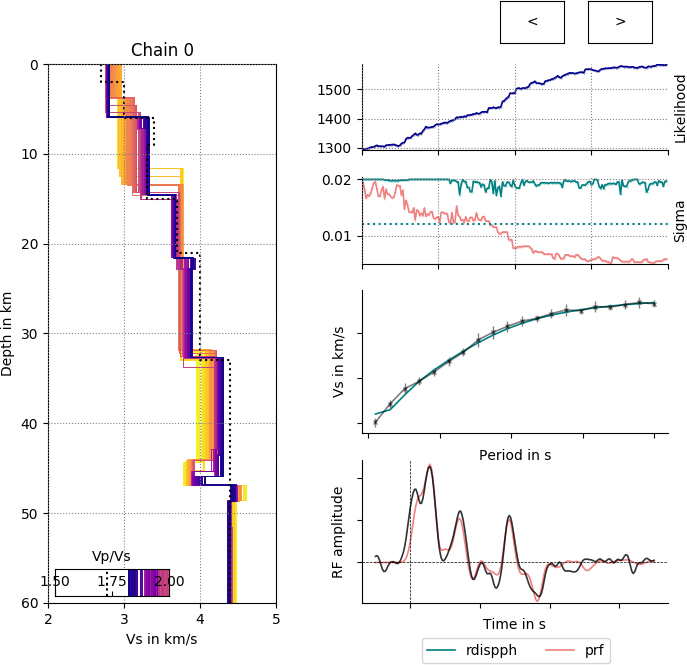
Screen shot of BayWatch live-stream showing the evolution of chain models with likelihood, i.e., the evolution of the \(\mathrm{V_S}\)-depth structure, \(\mathrm{V_P}\)/\(\mathrm{V_S}\) (with the darkest colored model being the current model) and \(\sigma\) (sigma) for the two targets. The live-stream shows an inversion of synthetic data from a six-layer velocity-depth model as described in Testing with synthetic data. The Colored dotted lines represent the “true” model values.